Last Modified 20 February 2000
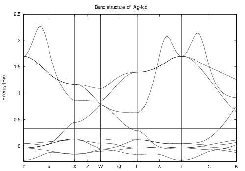
The previous pages in this example showed how to set up a SKIN file for band structure plotting and how to interpret the output. This page will show you how to actually plot the band structure from the QLMT file.
The form of the QLMT file is remarkably unsuitable for band structure plots. Thus we need a filter program to convert the QLMT file into something that a plotting program such as gnuplot can use. This is provided by the auxillary program bandplot.f.
In order to run bandplot, we need two input files; bandplot.in and dosdat.in.
The bandplot.in file format is listed below. You will notice that the QLMT we generated earlier is listed as an input file to be parsed by bandplot.The Fermi energy (0.32754) is provided for you, but Example 12 will show you how to calculate it for yourself. For the fcc configuration, the bandplot program requires 5 k-point directions. Finally, we specify our output files. The banddata output is the converted QLMT file, and the bandplot.gnu file is the generated gnuplot script that will create a file band.eps containing the band structure plot.
Ag-fcc
2
QLMT                                         ! Input file
PRIMITIVE VECTORS OF THE DIRECT LATTICE
  0.5  0.5  0.0
  0.5  0.0  0.5
  0.0  0.5  0.5
Number of bands to be ploted, maximum eigenvalue
9 100
Fermi energy (Ry)
   0.32754
Enter the number of k-directions in the Brillouin zone
5                                               ! k-directions in the Brillouin zone
 80                                             !number of k-point in the  1 direction
 40                                             !number of k-point in the  2 direction
 80                                             !number of k-point in the  3 direction
 80                                             !number of k-point in the  4 direction
 80                                             !number of k-point in the  5 direction
banddata                                       ! Output file -donot change the title
bandplot.gnu   					! Output gnuplot file
Compile bandplot.f, then run the executable.
$ ./bandplot
The output file, here banddata, has a rather simple form:
$ head -10 banddata

     0.000000    -0.277291    -0.038660    -0.038660    -0.038660     0.047466     0.047466     1.701297     1.701297     1.701297
     0.012658    -0.277162    -0.038710    -0.038610    -0.038610     0.047402     0.047491     1.701014     1.701014     1.702777
     0.025316    -0.276777    -0.038860    -0.038459    -0.038459     0.047213     0.047566     1.700163     1.700163     1.707211
     0.037974    -0.276135    -0.039109    -0.038208    -0.038208     0.046898     0.047691     1.698744     1.698744     1.714586
     0.050632    -0.275236    -0.039457    -0.037857    -0.037857     0.046460     0.047865     1.696757     1.696757     1.724880
     0.063292    -0.274080    -0.039903    -0.037405    -0.037405     0.045902     0.048089     1.694201     1.694201     1.738056
     0.075950    -0.272667    -0.040447    -0.036855    -0.036855     0.045228     0.048362     1.691076     1.691076     1.754066
     0.088608    -0.270996    -0.041087    -0.036205    -0.036205     0.044442     0.048683     1.687383     1.687383     1.772839
     0.101266    -0.269067    -0.041822    -0.035457    -0.035457     0.043549     0.049052     1.683122     1.683122     1.794285
     0.113924    -0.266882    -0.042651    -0.034611    -0.034611     0.042556     0.049468     1.678297     1.678297     1.818283
Each k-point in the QLMT file has its own line. The first number on the line represents the distance, in Cartesian reciprocal space, from the preceding k-point. The first point is arbitrarily assigned to be zero. If you'll go down to the 40th line of banddata you'll see the distance is 0.5, as it should be using this mesh, since according to our setup, it should be X.
Run
$ gnuplot bandplot.gnuto create the band structure plot.

Of course, the Fermi level in this graph was found by doing another calculation with a realistic k-point mesh, which you can read about in Example 12
Go back to the setup or output pages.
Look at other examples.
Return to the static Reference Manual.