Last Modified 15 February 2000

The ``Static'' Tight-Binding Program: Example VII

Although the true molecular dynamics programs on the DoD Tight-Binding Home Page can be used to obtain more structural information about a system more easily than static can, in one respect static is more useful, in that we can use it to look at the electronic band structure of a crystal. In this example, example 8, and example 9 we'll do just that.

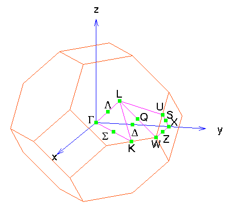
In this example we use our tight-binding parametrization to study the electronic structure of silver. In the ground state silver forms an fcc lattice, so its Brillouin zone is the same as the Wigner-Seitz cell of a bcc lattice. We'll plot the band structure along several lines connecting the high symmetry points of the Brillouin zone, as show in the figure below.

By now you know that the tight-binding parameters for silver can be obtained from the tight-binding periodic table under ``Ag'', and I'm sure you've saved these parameters in a working directory as ag_par.

The ground state of silver is the fcc lattice, so we'll steal the space group file from example 1 and rename it spcgrp.

We'll defer the discussion of the k-point ``mesh'' for a few moments.

We only one to calculate one band structure at a time, so the SKIN (Slater-Koster INput) file is rather simple in this case, except for the k-point mesh. Save this file in your working directory under the name SKIN, and then let's look at it in detail.

The first few lines of the file are slightly changed from previous examples:  

Mode=6               QLMT File
0.002  5.000         (T_{Fermi}, Eigenvalue cutoff for P calculation)
ag_par

Mode 6 tells the program to produce a QLMT file, a formatted list of the eigenvalues of the crystal at each k-point. When Mode=6, the static program only provides information about eigenvalues below the eigenvalue cutoff on line 2. Here we've set this to 5 Ry, which should allow us to plot all of the bands of silver. If we only wanted the eigenvalues near the Fermi level, we could make this number smaller, say 0.5, depending on the system.

Let's calculate the band structure at the experimental lattice constant of 4.09 Å =7.729 Bohr. Then the next part of the file is the reminiscent of example 1.

Silver FCC (A1) Band structure
 fcc  7.580          (20 character label for SKENG)
 0.00                (Electrons in addition to nominal Ag charge (=11/atom))
 1                   (fcc lattice, read in cubic lattice constant a)
 7.580               (lattice constant in Bohr)
 0                   (No additional strains applied)
 1                   (Atoms in the unit cell)
 4 4 4               (Neighbor search cutoff indices)
F                    (Logical variable -- no internal displacements)
 1  0.000  0.000  0.000  0 0 0   (Position of atom in Lattice coordinates)

The k-point generation routine is a little trickier. Well, the first part isn't any different than previous examples. We need to read in the space group file and tell the program that the file is in Cartesian coordinates:

NEWSYM=T (Generate new set of k-points)
LATTIC=1 (Lattice type / Next is spacegroup file name:)
spcgrp
ILAT=F (Space group file in Cartesian Coordinates)

As for the k-points themselves, we want to specify the k-points along some of the high-symmetry lines indicated in the Brillouin zone figure. The static program requires that we know the lattice coordinates of these lines, which means we need to know a little bit more about the lattice.

The lattice types table tells us that the ``standard'' primitive lattice vectors of the fcc lattice are

• a₁ = ( 0 , ½ a , ½ a)    
• a₂ = ( ½ a , 0 , ½ a)    
• a₃ = ( ½ a , ½ a , 0)   .

This means that the primitive vectors of the reciprocal lattice are specified by

• b₁ = 2 π ( -1/a , 1/a , 1/a)    
• b₂ = 2 π ( 1/a , -1/a , 1/a)    
• b₃ = 2 π ( 1/a , 1/a , -1/a)

In the table, X' is an equivalent point to X, and we leave it to the reader to show that K and U are equivalent.

So now we want to generate the k-points along the lines  

1. Gamma --> X via Delta
2. X --> W via Z
3. W --> L via Q
4. L --> Gamma via Lambda
5. Gamma --> K (=U) via Sigma

The k-point generating routine kptin.f has a special generating routine for such conditions. If the number of k-points is set equal to 999, then the program assumes that you are going to give it a set of directions along which it is to calculate the eigenvalues. Thus in this example we the following SKIN file fragment:

  999                 (K-points by direction)
    5                 (Number of directions)
 80 0.000 0.000 0.000  0.500 0.000 0.500  (Gamma -> Delta -> X)
 40 0.500 0.000 0.500  0.500 0.250 0.750  (X -> Z -> W)
 80 0.500 0.250 0.750  0.500 0.500 0.500  (W -> Q -> L)
 80 0.500 0.500 0.500  0.000 0.000 0.000  (L -> Lambda -> Gamma)
 80 0.000 0.000 0.000  0.375 0.375 0.750  (Gamma -> Sigma -> K(U))

The first line, 999, is as noted above. The next line (``5'') contains the number of lines which will be read in. Both lines must be in (I5) format. The following lines contain the directions, in the following format:

• The first number is the number of points along the line. Both end points count. Therefore the first line (Gamma -> Delta -> X) has 78 interior points.
• The next three columns give the lattice coordinates of one end of the line.
• The next three columns give the lattice coordinates of the other end of the line.
• These lines are read in under Fortran's ``free'' format.

The number of points you choose on a given line is a matter of taste. Too few points will give a choppy band structure, and too many points will take too long. The numbers here represent a compromise.

Now the program is ready to run.

Now go to the output discussion to see what will happen, or skip ahead to the band structure plot.

Look at other examples.

Get other parameters from the Tight-binding periodic table.

Return to the static Reference Manual.