Last Modified 17 December 1999

The ``Static'' Tight-Binding Program: Example VIII -- Output

Since we've discussed outputs of this type in detail in example 7 I'll speed things up considerably here.

If you've followed the steps on the setup page, then run the static code, your working directory should now look something like this:

$ ls -l
total 196
-rw-r--r--   1 mehl     users       93365 Jun  2 14:13 QLMT
-rw-r--r--   1 mehl     users          63 Jun  2 14:13 SKENG
-rw-r--r--   2 mehl     users        1305 Jun  2 14:12 SKIN
-rw-r--r--   1 mehl     users       29036 Jun  2 14:13 SKOUT
-rw-r--r--   1 mehl     users       43552 Jun  2 14:13 output
-r--r--r--   5 mehl     bind        10003 Aug 15  1996 spcgrp
-r--r--r--   3 mehl     users        7132 May 28 15:44 ta_par

where output is the standard output of static on this file.

Because of the weird k-point mesh, we don't expect SKENG to have the correct energy, and we're right:

 bcc equilibrium      121.251836    -.423478254 -779.936874125

The real interest in this static run is the QLMT file. We'll just look at the first k-point from this file:

    1    1    0    0     SPINS, WIND., SC. WIND.
  287 K-POINTS     1   5.00000    .00200
    .00000    .00000    .00000 287.00000         9    0.2870000000D+03 K
   -.4234783   0.000000E+00
    .2214703   0.000000E+00
    .2214703   0.000000E+00
    .2214703   0.000000E+00
    .4197155   0.000000E+00
    .4197155   0.000000E+00
   2.1965935   0.000000E+00
   2.1965935   0.000000E+00
   2.1965935   0.000000E+00

This looks much like the result in example 7, except that there is no angular momentum decomposition in this case, since we ran the calculation with Mode=9.

We can now run bandplot to convert the QLMT file into something we can plot. To do this, I'll again choose a ``lattice constant'' of 4Pi. This script will then produce file suitable for plotting:

bandplot << doneplot
QLMT
-6.283185307179586 6.283185307179586 6.283185307179586
6.283185307179586 -6.283185307179586 6.283185307179586
6.283185307179586 6.283185307179586 -6.283185307179586
0
1 9 100
ta.bands
doneplot

If you are trying to do this interactively, note that the proper response to the question ``How many atoms in a unit cell?'' is ``0''.

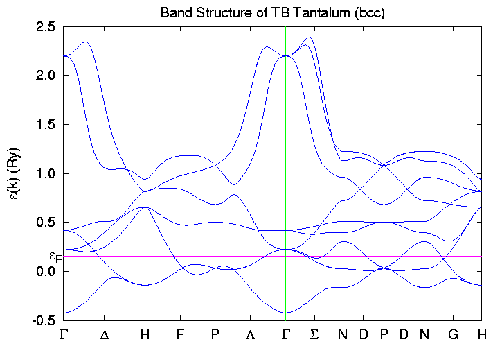
The gnuplot input to plot this file is similar to the previous example, so I'll just give you the script here. If you save it as ta.gnu, you'll get a reasonable plot. For a fancy plot with real Greek lettering, you'll need to use gnuplot's enhanced Postscript ``terminal''. When you do that, you'll get a plot like

Of course, the Fermi level in this graph was found by doing another calculation with a realistic k-point mesh.

Go back to the setup.

Look at other examples.

Return to the static Reference Manual.