Last Modified 17 December 1999
If you've followed the steps on the setup page, your working directory should now look something like this:
$ ls -l
total 72
-rw-r--r--   2 mehl     usr         7990 May 27 16:32 SKIN
-r--r--r--   2 mehl     usr         7196 May 26 11:15 cu_par
-r--r--r--   2 mehl     usr        13755 May 26 11:15 fcccp.08
-rw-r--r--   3 mehl     bind        1742 May 26 13:36 spcgrp
Now run the static code in this directory. You'll get something like this:
$ static > output
$ ls -l
total 256
-rw-r--r--   1 mehl     bind         693 May 27 16:36 SKENG
-rw-r--r--   2 mehl     usr         7990 May 27 16:32 SKIN
-rw-r--r--   1 mehl     bind       48837 May 27 16:36 SKOUT
-r--r--r--   2 mehl     usr         7196 May 26 11:15 cu_par
-r--r--r--   2 mehl     usr        13755 May 26 11:15 fcccp.08
-rw-r--r--   1 mehl     bind       38550 May 27 16:36 output
-rw-r--r--   3 mehl     bind        1742 May 26 13:36 spcgrp
As usual, we are most interested in the SKENG file:
 e1^2= 0.0000          79.373431     .223123231     .002522352
 e1^2= 0.0001          79.373431     .223478107     .002548645
 e1^2= 0.0005          79.373431     .225726005     .002701642
 e1^2= 0.0010          79.373431     .227837078     .002895057
 e1^2= 0.0020          79.373431     .229384227     .003168428
 e1^2= 0.0025          79.373431     .229443780     .003282096
 e1^2= 0.0030          79.373431     .229938416     .003404008
 e1^2= 0.0040          79.373431     .231513566     .003659530
 e1^2= 0.0050          79.373431     .232441293     .003876163
 e1^2= 0.0075          79.373431     .234226500     .004433613
 e1^2= 0.0100          79.373431     .233982214     .004924936
Note that the energy increases monotonically with strain, which is a good thing, as otherwise the fcc phase would not be the ground state. Now remember that Equation 2 tells us that the energy E should be close to a linear function of the squared strain e12. To see this, let's drag out gnuplot:
$ gnuplot

        G N U P L O T
        Linux version 3.5 (pre 3.6)
        patchlevel beta 340
        last modified Tue Nov 25 22:57:44 GMT 1997

        Copyright(C) 1986 - 1993, 1997
        Thomas Williams, Colin Kelley and many others

        Send comments and requests for help to info-gnuplot@dartmouth.edu
        Send bugs, suggestions and mods to bug-gnuplot@dartmouth.edu

Terminal type set to 'x11'
gnuplot> set format x "%.3f"
gnuplot> set format y "%.4f"
gnuplot> set xrange [0:0.0105]
gnuplot> plot "SKENG" using 2:5 notitle w linesp
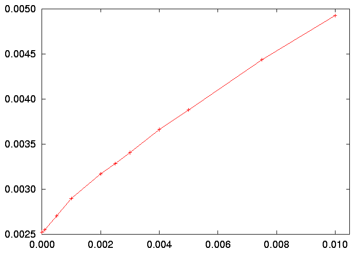
which produces the graph:

This is a little ragged, but we should be able to get a reasonable fit to the data. First we note that the 3.6 beta version of gnuplot allows us to write a more or less arbitrary function with up to five variables. From Equation 2 we see that a reasonable function to fit is
Note that in (3) we know the volume V, and want to determine the remaining parameters E0, C11-C12, a, and b to best fit the data in SKENG.
The gnuplot script cufit.gnu is designed to do this fit. Let's run it:
$ gnuplot cufit.gnu Current Volume is 79.373431 Correct if necessary Pressto continue [If the volume is not correct, edit cufit.gnu to fix it.] [fitting information deleted. See fit.log.] Found C_{11} - C_{12} = 63.7897462764449 GPa at V = 79.373431 Bohr^3 Press to conclude
The fit finds (C11-C12) = 64 GPa. This should be compared to the experimental value of 47 GPa and the first-principles value of 50 &GPa. Our fit is a little stiff, but not too bad.
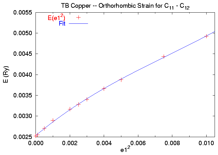
cufit.gnu also produces a gnuplot file cuplot.gnu, which can be used as the basis of a publication quality plot. Using the gif option of gnuplot we get to take a look at the points and the fit together.

This should give you some idea of the accuracy of the fit.
Return to the setup page.
Look at other examples.
Get other parameters from the Tight-binding periodic table.
Return to the static Reference Manual.