Last updated -- 17 December 1999
On the previous page we showed how to set up the Slater-Koster INput (SKIN) file to determine the energy of a Titanium hcp lattice at fixed volume and changing c/a. If you've followed all of the steps there, your working directory should look something like this:
$ ls -l
total 48
-rw-r-----   2 mehl     usr         9388 May 26 09:04 SKIN
-r--r--r--  10 mehl     bind        1511 Jul 28 1997  spcgp1.hcp
-r--r-----   2 mehl     usr         7127 May 26 09:04 ti_par
Running the SKIN file will produce some standard output, more information in the SKOUT file, and the SKENG file, which looks like this:
 hcp  1.30      238.000000     .117314145     .024705471
 hcp  1.35      238.000000     .119581774     .016649309
 hcp  1.40      238.000000     .121556959     .009891193
 hcp  1.45      238.000000     .122982153     .004410630
 hcp  1.50      238.000000     .123637708     .000258016
 hcp  1.55      238.000000     .123556447    -.002424527
 hcp  1.60      238.000000     .122991475    -.003531013
 hcp  1.65      238.000000     .122139102    -.003022974
 hcp  1.70      238.000000     .121017689    -.000979273
 hcp  1.75      238.000000     .119708601     .002346331
 hcp  1.80      238.000000     .118372237     .006771372
 hcp  1.85      238.000000     .117046651     .012002014
 hcp  1.90      238.000000     .116008367     .017698929
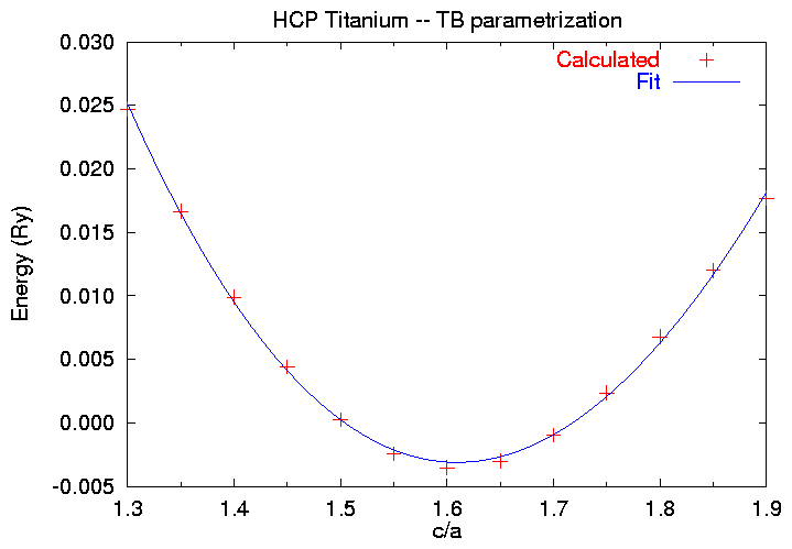
Each line represents one calculation. The first two columns are part of the label from the SKIN file, the next column is the Volume, followed by the Fermi energy in Rydbergs, and then the energy in Rydbergs. We see that the equilibrium c/a ratio is about 1.6. This is a bit larger than the experimental c/a value of 1.586, but not too bad.
To find a better approximation to the minimum energy c/a ratio,
we can use the gnuplot scripte tifit.gnu, which fits the above
information to the functional form
Running the script tifit.gnu
(which saves itself in tiplot.gnu)
produces this graph:

along with the output:
$ gnuplot tifit.gnu
[Fitting information log file deleted]
Equilibrium c/a ratio = 1.60927506481414
As we can see from the graph, the fit isn't terribly good, but it is a start. Example 10 will show a ``quick and dirty'' way of determining the equilibrium c/a ratio to arbitrary accuracy.
Go back to the setup page.
Look at other examples.
Return to the static Reference Manual.