Last Modified 17 December 1999

The ``Static'' Tight-Binding Program: Example X

Monoclinic strain to find C₄₄ -- Fully Relaxed

Theory

The calculations shown on this page determine the fully relaxed elastic constant C₄₄. I've also written a page which shows how to calculate the upper bound of C₄₄. This page also explains the theory.

The theory for determining the fully relaxed elastic constant C₄₄ of an hcp lattice is worked out as part of the upper bound calculation. What we need to know from the theory is that

Strain type 6 in the predefined strain table gives:
e₄ = x ; e₃ = + ¼ x² ; e_1,2,5,6 = 0 . (1)

This is a volume conserving strain which has the nice property that E(-x) = E(x) for an hcp lattice. Therefore the energy/strain relationship is
E(x) = E₀ + ½ V₀ C₄₄ x² + O[x⁴] (2)
In this case the strained hcp lattice then has the form

a₁ = ( ½ a , - ½ 3^½ a , - ¼ 3^½ x a )

a₂ = ( ½ a , ½ 3^½ a , ¼ 3^½ x a ) . (3)

a₃ = ( 0 , ½ x c , ( 1 + ¼ x² ) c )

With symmetry turns out to be C2/m (#12 in the International Crystallography tables), a centered monoclinic lattice with the atoms sitting on the 4m sites. The basis vectors can be written in the form

B₁ = (1/3 - u) a₁ + (2/3 + u) a₂ + (1/4 + v) a₃

B₂ = (2/3 + u) a₁ + (1/3 - u) a₂ + (3/4 - v) a₃ , (4)

where u and v are free parameters. (It's best not to look at the Cartesian expressions for these vectors.) Note that when x=0, we only get back to the hcp lattice when we also have u=v=0.

Just as in the case of the upper bound calculation, we need

The space group file for C2/m, which I've put in work/c44r/spcgp1.12 .
The k-point file, which is now in work/c44r/kmesh.12 .

Algorithm

The algorithm we'll use here is similar to what we did in the equation of state and C₁₁-C₁₂ calculations: at a given strain, we make a guess at the internal parameters (u,v), calculate E at several points near this guess, and use these values to determine a guess at the equilibrium configuration. Unlike the previous examples, we now have two variables. So, assuming that we are close to the minimum structure, which is probably near (u,v) = (1/3,/14), we fit our data to a quadratic polynomial:

E(u,v) = a + b u + c v + d u² + e v² + f u v . (5)
Obviously this requires a minimum of six points. We'll use the original point (u,v) and five points equally spaced on a circle of radius h around (u,v).

The script which does the fitting is called work/c44r/minlat . It requires input of

The volume of the primitive cell
The c/a ratio
The square of the strain parameter, x²
The radius h of the circle
A guess at u_min
A guess at v_min

The output is

The volume of the primitive cell
The c/a ratio
The square of the strain parameter, x²
The radius h of the circle
A new guess at u_min
A new guess at v_min
A guess at the energy of this new structure.

Let's look at an example. Before starting, edit your copy of work/c44r/minlat so that the variable $static, defined here as

static=/usr/local/mehl/skfits/p6/static.105/static

points to the location of your static executable.

We'll use the TB equilibrium lattice of

V = 220.088 Bohr³
c/a = 1.6132603 .

As an initial guess, a step size h = 0.01 should be OK, but we can change it as we go if necessary.

First let's see if we get the correct structure at zero strain.

$ ./minlat 220.088 1.6132603 0.0000 0.01 0.3333333333333333333  0.25
 1 0.333333 0.250000  220.088000     .128472502    -.009018141
 2 0.343333 0.250000  220.088000     .127977634    -.008038481
 3 0.336424 0.259511  220.088000     .129657127    -.006448887
 4 0.325243 0.255878  220.088000     .128592230    -.007510231
 5 0.325243 0.244122  220.088000     .128592230    -.007510231
 6 0.336424 0.240489  220.088000     .129657127    -.006448887
220.088 1.6132603 0.0000 0.010000000000000 0.333058297294762 0.250000000000000 -0.009018843
[Note:  I may have overdone the precision. -- mjm]

The first six lines are the actual energies calculated by the static code. The last line is the prediction. If one of the first second through sixth energies is lower in energy than the predicted minimum then you have not bracketed the minimum correctly, and should restart the calculation.

Note that the prediction is off from our expectations, and is, in fact, larger than the initial energy. In this case it means that we have made h too large. Try again:

$ ./minlat 220.088 1.6132603 0.0000 0.001 0.3333333333333333333 0.25
 1 0.333333 0.250000  220.088000     .128472502    -.009018141
 2 0.334333 0.250000  220.088000     .128467360    -.009008840
 3 0.333642 0.250951  220.088000     .128484739    -.008993074
 4 0.332524 0.250588  220.088000     .128473968    -.009002893
 5 0.332524 0.249412  220.088000     .128473968    -.009002893
 6 0.333642 0.249049  220.088000     .128484739    -.008993074
220.088 1.6132603 0.0000 0.001000000000000 0.333330707514992 0.250000000000000 -0.009018141

This is somewhat better.

You'll notice that this calculation leaves a file work/c44r/skeng.0.0000. Runs for other strains will leave a similar set of calculations. For example, at the strain x² = 0.0010 we have the file work/c44r/skeng.0.0010:

 1 0.333333 0.250000  220.088000     .128082626    -.008489157
 2 0.334333 0.250000  220.088000     .128079535    -.008473758
 3 0.333642 0.250951  220.088000     .128095218    -.008459921
 4 0.332524 0.250588  220.088000     .128084009    -.008479995
 5 0.332524 0.249412  220.088000     .128081551    -.008477608
 6 0.333642 0.249049  220.088000     .128095701    -.008464184
 1 0.332999 0.250004  220.088000     .128081472    -.008490171
 2 0.333999 0.250004  220.088000     .128081651    -.008480962
 3 0.333308 0.250955  220.088000     .128095853    -.008463857
 4 0.332190 0.250592  220.088000     .128080649    -.008476702
 5 0.332190 0.249416  220.088000     .128077226    -.008473098
 6 0.333308 0.249053  220.088000     .128094797    -.008466077
 1 0.332998 0.250004  220.088000     .128081463    -.008490171 < Lowest energy
 2 0.333998 0.250004  220.088000     .128081659    -.008480993
 3 0.333307 0.250955  220.088000     .128095858    -.008463864
 4 0.332189 0.250592  220.088000     .128080631    -.008476676
 5 0.332189 0.249416  220.088000     .128077199    -.008473075
 6 0.333307 0.249053  220.088000     .128094785    -.008466089

From this output you should be able to retrace my route and find that the lowest energy for this strain is -.008490171 Ry.

To get a good estimate of C₄₄ we need to look at several strains, though not necessarily as many as we did in the upper bound calculation. I'll list all of the results here:

$ ls skeng.*
-rw-r-----   1 mehl     users         756 Jun 23 15:31 skeng.0.0000
-rw-r-----   1 mehl     users        1134 Jun 23 15:44 skeng.0.0010
-rw-r-----   1 mehl     users        1134 Jun 23 15:53 skeng.0.0020
-rw-r-----   1 mehl     users        1134 Jun 23 16:05 skeng.0.0030
-rw-r-----   1 mehl     users        1134 Jun 23 16:15 skeng.0.0040
-rw-r-----   1 mehl     users        1134 Jun 23 16:26 skeng.0.0050

We now need a way to extract the minimum energy from each these files and put the results in a file which will give us the minimum energy at each strain. This script is work/c44r/findmin , a variant of other findmin scripts in this Example. Note that, as usual, findmin depends on the sort routine. As mentioned in the comments, the GNU version of this routine has trouble when we mix positive and negative numbers. This won't be a problem in this example, but look out in other cases.

findmin produces the file work/c44r/c44.eng, which looks like this:

0.0000 0.333333 0.250000 220.088000 .128472502 -.009018141
0.0010 0.332998 0.250004 220.088000 .128081463 -.008490171
0.0020 0.332629 0.250020 220.088000 .127697318 -.007960869
0.0030 0.332226 0.250046 220.088000 .127318114 -.007433716
0.0040 0.331794 0.250082 220.088000 .126941539 -.006910690
0.0050 0.331338 0.250126 220.088000 .126566240 -.006392912

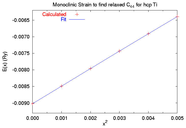
The fitting process is nearly identical to the upper bound calculation. Here we use the gnuplot script work/c44r/c44fit.gnu to find

$ gnuplot c44fit.gnu
Using eo = -0.009018141 vo = 220.088
Edit c44fit.gnu to change
Press enter to continue
Fitting information deleted, see work/c44r/fit.log
C_{44} = 70.3060841127926 GPa
Press enter to quit
(script work/c44r/c44.gnu prepared)

and

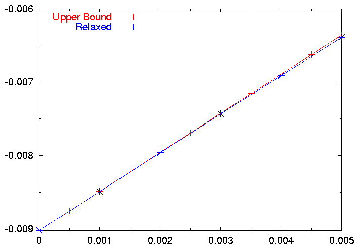
We see that the elastic constant here is slightly larger than the elastic constant in the upper bound calculation. This is a result of our not fitting quite the same number of points. It is instructive to compare the two results. This plot was produced by the script work/c44r/c44comp.gnu:

Comparison of relaxed and upper bound
calculations

The relaxed data is just below the upper bound calculation, as it should be. Clearly, though, there is very little relaxation in this lattice, and we can safely say that

C₄₄ = 70.3 GPa

for our hcp Titanium parameters.

Look at the Upper Bound calculation and the theory for calculation of C₄₄ in an hcp lattice.

Go back to the Example X home page.

Look at other examples.

Get other parameters from the Tight-binding periodic table.

static Home Page Introduction About Version 1.11 Installation List of Files Usage Input Files Output Files Trouble Shooting Appendix

Return to the static Reference Manual.

a₁	= (	½ a ,	- ½ 3^½ a ,	- ¼ 3^½ x a )
a₂	= (	½ a ,	½ 3^½ a ,	¼ 3^½ x a )	. (3)
a₃	= (	0 ,	½ x c ,	( 1 + ¼ x² ) c )

B₁	=	(1/3 - u) a₁ + (2/3 + u) a₂ + (1/4 + v) a₃
B₂	=	(2/3 + u) a₁ + (1/3 - u) a₂ + (3/4 - v) a₃	, (4)

Last Modified 17 December 1999

The ``Static'' Tight-Binding Program: Example X

Monoclinic strain to find C44 -- Fully Relaxed

Theory

Algorithm

Monoclinic strain to find C₄₄ -- Fully Relaxed