Last Modified 17 December 1999

The ``Static'' Tight-Binding Program: Example X

Change in energy as a function of c at fixed a

So far we've looked at the energy of the hcp Titanium lattice as a function of

We can exploit one more strain which keeps the full P6₃/mmc symmetry of the hcp lattice. In this case we fix the lattice constant a and allow c to vary:

c ---> c' = c (1 + z) , (1)

then according to our elastic constant tutorial we've constructed a strain

e_1,2 = 0 ; e₃ = z ; e_4-6 = 0 , (2)

which leads to the energy-strain relationship

E(z) = E₀ + ½ V₀ C₃₃ z² + O[z³] (3)

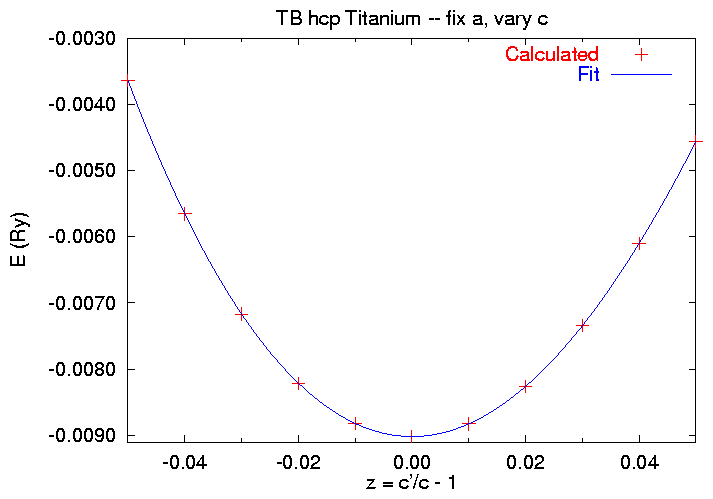
So now we: calculate E(z) at several points z, and determine the the elastic constant from a polynomial fit to the data. We'll do this in the directory work/c33. Again, the pre-defined strain types table does not have an entry for the strain (2), so we'll have to use option ``1'' and provide all six of the e_i. Thus the first calculation in the work/c33/SKIN file looks like this:

Mode=3               (Calculate energy only -- no pressure)
0.005  0.500         (T_{Fermi}, Eigenvalue cutoff for P calculation)
../ti_par
Titanium HCP (A3) -- Fixed a
 1.61326030 -0.050   (We'll use the label to indicate c/a and strain)
 0.00                (Electrons in addition to nominal Ti charge (=4/atom))
-3                   (hexagonal lattice, read in V and c/a)
 220.088  1.61326030 (V in Bohr^3 and c/a)
 1                   (General strain)
 0 0 -0.050 0 0 0    (the strain factors)
 2                   (Atoms in the unit cell)
 4 4 4               (Neighbor search cutoff indices)
F                    (Logical variable -- no internal displacements)
1 0.33333333333333333 0.66666666666666667 0.25 0 0 0   (Atom 1 in lattice coord.)
1 0.66666666666666667 0.33333333333333333 0.75 0 0 0   (Atom 2 in lattice coord.)
NEWSYM=T             (Generate new set of k-points)
LATTIC=4             (Lattice type / Next is spacegroup file name:)
../spcgp1.hcp
ILAT=T               (Space group file in lattice Coordinates)
-1313                (Read k-point generation information from file)
../kmesh.194

We use strain option 1, so we have to specify all six e_i, according to (2). When we run the code for a full set of strains, we find

$ cat SKENG
 1.61326030 -0.050    209.083600     .134069317    -.003642696
 1.61326030 -0.040    211.284480     .133000251    -.005655484
 1.61326030 -0.030    213.485360     .131907130    -.007168730
 1.61326030 -0.020    215.686240     .130779913    -.008212985
 1.61326030 -0.010    217.887120     .129627497    -.008820742
 1.61326030  0.000    220.088000     .128472502    -.009018141
 1.61326030  0.010    222.288880     .127334905    -.008825389
 1.61326030  0.020    224.489760     .126223305    -.008260279
 1.61326030  0.030    226.690640     .125131816    -.007343170
 1.61326030  0.040    228.891520     .124050273    -.006100872
 1.61326030  0.050    231.092400     .122978185    -.004563108

We'll use a modification of the fitting procedure we used in E(a) at fixed c case, using gnuplot to fit this data to the polynomial

E(x) = E₀ + ½ V₀ x² [ C₃₃ + x ( A + x ( B + x C))] , (4)

where A, B, and C are higher order elastic constants. When we run the fitting script we get

$ gnuplot c33fit.gnu 
Starting from v0 = 220.088 and e0 = -0.009018141
Change if appropriate
Press  to continue
[Fitting information deleted.  See fit.log]
C_{33} = 261.217391809226 GPa
Press  to quit
$

and the graph looks like this: E(c) at fixed a for hcp Ti

So in this section we've found that

C₃₃ = 261.2 GPa

Go back to the Example X home page.

Look at other examples.

Get other parameters from the Tight-binding periodic table.

static Home Page Introduction About Version 1.11 Installation List of Files Usage Input Files Output Files Trouble Shooting Appendix

Return to the static Reference Manual.